《机器学习》学习笔记(二):神经网络
来源:程序员人生 发布时间:2015-03-11 08:44:46 阅读次数:3844次
在解决1些简单的分类问题时,线性回归与逻辑回归就足以应付,但面对更加复杂的问题时(例如对图片中车的类型进行辨认),应用之前的线性模型可能就得不到理想的结果,而且由于更大的数据量,之前方法的计算量也会变得异常庞大。因此我们需要学习1个非线性系统:神经网络。
我在学习时,主要通过Andrew Ng教授提供的网络,而且文中多处都有鉴戒Andrew Ng教授在mooc提供的资料。
转载请注明出处:http://blog.csdn.net/u010278305
神经网络在解决1些复杂的非线性分类问题时,相对线性回归、逻辑回归,都被证明是1个更好的算法。其实神经网络也能够看作的逻辑回归的组合(叠加,级联等)。
1个典型神经网络的模型以下图所示:
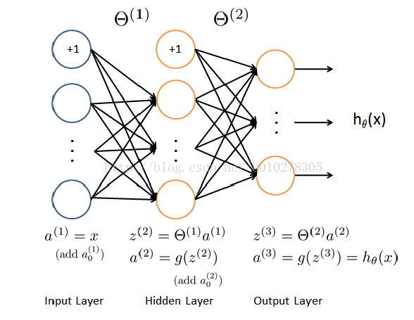
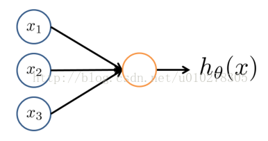
上述模型由3个部份组成:输入层、隐藏层、输出层。其中输入层输入特点值,输出层的输出作为我们分类的根据。例如1个20*20大小的手写数字图片的辨认举例,那末输入层的输入即可以是20*20=400个像素点的像素值,即模型中的a1;输出层的输出即可以看作是该幅图片是0到9其中某个数字的几率。而隐藏层、输出层中的每一个节点其实都可以看作是逻辑回归得到的。逻辑回归的模型可以看作这样(以下图所示):
有了神经网络的模型,我们的目的就是求解模型里边的参数theta,为此我们还需知道该模型的代价函数和每个节点的“梯度值”。
代价函数的定义以下:

代价函数关于每个节点处theta的梯度可以用反向传播算法计算出来。反向传播算法的思想是由于我们没法直观的得到隐藏层的输出,但我们已知输出层的输出,通过反向传播,倒退其参数。
我们以以下模型举例,来讲明反向传播的思路、进程:
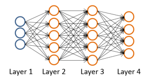
该模型与给出的第1个模型不同的是,它具有两个隐藏层。
为了熟习这个模型,我们需要先了解前向传播的进程,对此模型,前向传播的进程以下:
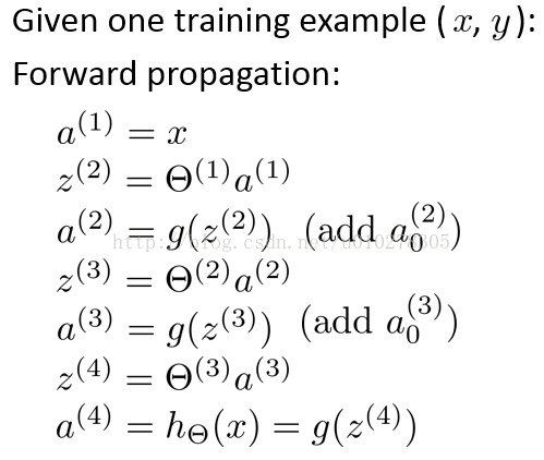
其中,a1,z2等参数的意义可以参照本文给出的第1个神经网络模型,类比得出。
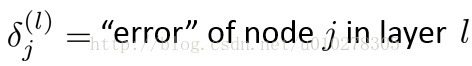
然后我们定义误差delta符号具有以下含义(以后推导梯度要用):
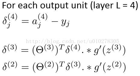
误差delta的计算进程以下:
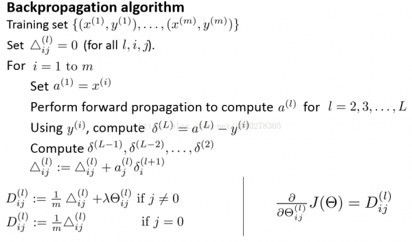
然后我们通过反向传播算法求得节点的梯度,反向传播算法的进程以下:
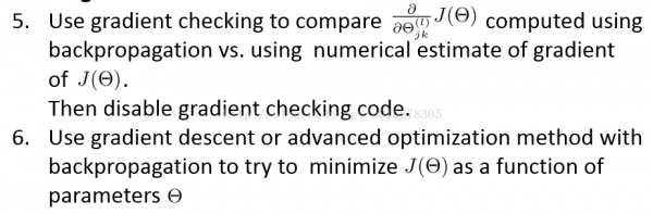
有了代价函数与梯度函数,我们可以先用数值的方法检测我们的梯度结果。以后我们就能够像之前那样调用matlab的fminunc函数求得最优的theta参数。
需要注意的是,在初始化theta参数时,需要赋予theta随机值,而不能是固定为0或是甚么,这就避免了训练以后,每一个节点的参数都是1样的。
下面给出计算代价与梯度的代码:
function [J grad] = nnCostFunction(nn_params, ...
input_layer_size, ...
hidden_layer_size, ...
num_labels, ...
X, y, lambda)
%NNCOSTFUNCTION Implements the neural network cost function for a two layer
%neural network which performs classification
% [J grad] = NNCOSTFUNCTON(nn_params, hidden_layer_size, num_labels, ...
% X, y, lambda) computes the cost and gradient of the neural network. The
% parameters for the neural network are "unrolled" into the vector
% nn_params and need to be converted back into the weight matrices.
%
% The returned parameter grad should be a "unrolled" vector of the
% partial derivatives of the neural network.
%
% Reshape nn_params back into the parameters Theta1 and Theta2, the weight matrices
% for our 2 layer neural network
Theta1 = reshape(nn_params(1:hidden_layer_size * (input_layer_size + 1)), ...
hidden_layer_size, (input_layer_size + 1));
Theta2 = reshape(nn_params((1 + (hidden_layer_size * (input_layer_size + 1))):end), ...
num_labels, (hidden_layer_size + 1));
% Setup some useful variables
m = size(X, 1);
% You need to return the following variables correctly
J = 0;
Theta1_grad = zeros(size(Theta1));
Theta2_grad = zeros(size(Theta2));
% ====================== YOUR CODE HERE ======================
% Instructions: You should complete the code by working through the
% following parts.
%
% Part 1: Feedforward the neural network and return the cost in the
% variable J. After implementing Part 1, you can verify that your
% cost function computation is correct by verifying the cost
% computed in ex4.m
%
% Part 2: Implement the backpropagation algorithm to compute the gradients
% Theta1_grad and Theta2_grad. You should return the partial derivatives of
% the cost function with respect to Theta1 and Theta2 in Theta1_grad and
% Theta2_grad, respectively. After implementing Part 2, you can check
% that your implementation is correct by running checkNNGradients
%
% Note: The vector y passed into the function is a vector of labels
% containing values from 1..K. You need to map this vector into a
% binary vector of 1's and 0's to be used with the neural network
% cost function.
%
% Hint: We recommend implementing backpropagation using a for-loop
% over the training examples if you are implementing it for the
% first time.
%
% Part 3: Implement regularization with the cost function and gradients.
%
% Hint: You can implement this around the code for
% backpropagation. That is, you can compute the gradients for
% the regularization separately and then add them to Theta1_grad
% and Theta2_grad from Part 2.
%
J_tmp=zeros(m,1);
for i=1:m
y_vec=zeros(num_labels,1);
y_vec(y(i))=1;
a1 = [ones(1, 1) X(i,:)]';
z2=Theta1*a1;
a2=sigmoid(z2);
a2=[ones(1,size(a2,2)); a2];
z3=Theta2*a2;
a3=sigmoid(z3);
hThetaX=a3;
J_tmp(i)=sum(-y_vec.*log(hThetaX)-(1-y_vec).*log(1-hThetaX));
end
J=1/m*sum(J_tmp);
J=J+lambda/(2*m)*(sum(sum(Theta1(:,2:end).^2))+sum(sum(Theta2(:,2:end).^2)));
Delta1 = zeros( hidden_layer_size, (input_layer_size + 1));
Delta2 = zeros( num_labels, (hidden_layer_size + 1));
for t=1:m
y_vec=zeros(num_labels,1);
y_vec(y(t))=1;
a1 = [1 X(t,:)]';
z2=Theta1*a1;
a2=sigmoid(z2);
a2=[ones(1,size(a2,2)); a2];
z3=Theta2*a2;
a3=sigmoid(z3);
delta_3=a3-y_vec;
gz2=[0;sigmoidGradient(z2)];
delta_2=Theta2'*delta_3.*gz2;
delta_2=delta_2(2:end);
Delta2=Delta2+delta_3*a2';
Delta1=Delta1+delta_2*a1';
end
Theta1_grad=1/m*Delta1;
Theta2_grad=1/m*Delta2;
Theta1(:,1)=0;
Theta1_grad=Theta1_grad+lambda/m*Theta1;
Theta2(:,1)=0;
Theta2_grad=Theta2_grad+lambda/m*Theta2;
% -------------------------------------------------------------
% =========================================================================
% Unroll gradients
grad = [Theta1_grad(:) ; Theta2_grad(:)];
end
最后总结1下,对1个典型的神经网络,训练进程以下:
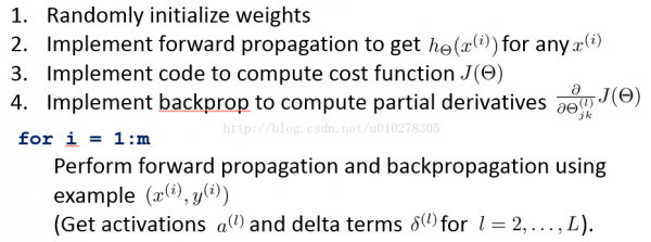
依照这个步骤,我们就能够求得神经网络的参数theta。
转载请注明出处:http://blog.csdn.net/u010278305
生活不易,码农辛苦
如果您觉得本网站对您的学习有所帮助,可以手机扫描二维码进行捐赠