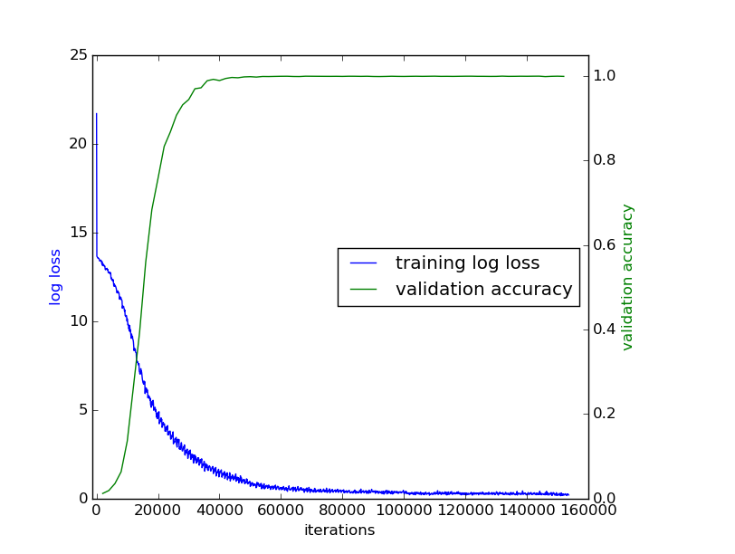
当我们设计好网络结构后,在神经网络训练的进程中,迭代输出的log信息中,1般包括,迭代次数,训练损失代价,测试损失代价,测试精度等。本文提供1段示例,简单讲述如何绘制训练曲线(training curve)。
首先看1段训练的log输出,网络结构参数的那段疏忽,直接跳到训练迭代阶段:
I0627 21:30:06.004370 15558 solver.cpp:242] Iteration 0, loss = 21.6953
I0627 21:30:06.004420 15558 solver.cpp:258]     Train net output #0: loss = 21.6953 (* 1 = 21.6953 loss)
I0627 21:30:06.004426 15558 solver.cpp:571] Iteration 0, lr = 0.01
I0627 21:30:28.592690 15558 solver.cpp:242] Iteration 100, loss = 13.6593
I0627 21:30:28.592730 15558 solver.cpp:258]     Train net output #0: loss = 13.6593 (* 1 = 13.6593 loss)
I0627 21:30:28.592733 15558 solver.cpp:571] Iteration 100, lr = 0.01

...

I0627 21:37:47.926597 15558 solver.cpp:346] Iteration 2000, Testing net (#0)
I0627 21:37:48.588079 15558 blocking_queue.cpp:50] Data layer prefetch queue empty
I0627 21:40:40.575474 15558 solver.cpp:414]     Test net output #0: loss = 13.07728 (* 1 = 13.07728 loss)
I0627 21:40:40.575477 15558 solver.cpp:414]     Test net output #1: loss/top⑴ = 0.00226
I0627 21:40:40.575487 15558 solver.cpp:414]     Test net output #2: loss/top⑸ = 0.01204
I0627 21:40:40.708261 15558 solver.cpp:242] Iteration 2000, loss = 13.1739
I0627 21:40:40.708302 15558 solver.cpp:258]     Train net output #0: loss = 13.1739 (* 1 = 13.1739 loss)
I0627 21:40:40.708307 15558 solver.cpp:571] Iteration 2000, lr = 0.01

...

I0628 01:28:47.426129 15558 solver.cpp:242] Iteration 49900, loss = 0.960628
I0628 01:28:47.426177 15558 solver.cpp:258]     Train net output #0: loss = 0.960628 (* 1 = 0.960628 loss)
I0628 01:28:47.426182 15558 solver.cpp:571] Iteration 49900, lr = 0.01
I0628 01:29:10.084050 15558 solver.cpp:449] Snapshotting to binary proto file train_net/net_iter_50000.caffemodel
I0628 01:29:10.563587 15558 solver.cpp:734] Snapshotting solver state to binary proto filetrain_net/net_iter_50000.solverstate
I0628 01:29:10.692239 15558 solver.cpp:346] Iteration 50000, Testing net (#0)
I0628 01:29:13.192075 15558 blocking_queue.cpp:50] Data layer prefetch queue empty
I0628 01:31:00.595120 15558 solver.cpp:414]     Test net output #0: loss = 0.6404232 (* 1 = 0.6404232 loss)
I0628 01:31:00.595124 15558 solver.cpp:414]     Test net output #1: loss/top⑴ = 0.953861
I0628 01:31:00.595127 15558 solver.cpp:414]     Test net output #2: loss/top⑸ = 0.998659
I0628 01:31:00.727577 15558 solver.cpp:242] Iteration 50000, loss = 0.680951
I0628 01:31:00.727618 15558 solver.cpp:258]     Train net output #0: loss = 0.680951 (* 1 = 0.680951 loss)
I0628 01:31:00.727623 15558 solver.cpp:571] Iteration 50000, lr = 0.0096这是1个普通的网络训练输出,含有1个loss,可以看出solver.prototxt的部份参数为:
test_interval: 2000
base_lr: 0.01
lr_policy: "step" # or "multistep"
gamma: 0.96
display: 100
stepsize: 50000 # if is "multistep", the first stepvalue is set as 50000
snapshot_prefix: "train_net/net"
固然,上面的分析,即使不理睬,对下面的代码也没甚么影响,绘制训练曲线本质就是文件操作,从上面的log文件中,我们可以看出:
] Iteration和loss =的文本行,含有训练的迭代次数和损失代价;] Iteration和Testing net (#0)的文本行,含有测试的对应的训练迭代次数;#2:和loss/top⑸的文本行,含有测试top⑸的精度。根据这些分析,就能够对文本进行以下处理:
import os
import sys
import numpy as np
import matplotlib.pyplot as plt
import math
import re
import pylab
from pylab import figure, show, legend
from mpl_toolkits.axes_grid1 import host_subplot

# read the log file
fp = open('log.txt', 'r')

train_iterations = []
train_loss = []
test_iterations = []
test_accuracy = []

for ln in fp:
  # get train_iterations and train_loss
  if '] Iteration ' in ln and 'loss = ' in ln:
    arr = re.findall(r'ion \b\d+\b,',ln)
    train_iterations.append(int(arr[0].strip(',')[4:]))
    train_loss.append(float(ln.strip().split(' = ')[-1]))
  # get test_iteraitions
  if '] Iteration' in ln and 'Testing net (#0)' in ln:
    arr = re.findall(r'ion \b\d+\b,',ln)
    test_iterations.append(int(arr[0].strip(',')[4:]))
  # get test_accuracy
  if '#2:' in ln and 'loss/top⑸' in ln:
    test_accuracy.append(float(ln.strip().split(' = ')[-1]))

fp.close()

host = host_subplot(111)
plt.subplots_adjust(right=0.8) # ajust the right boundary of the plot window
par1 = host.twinx()
# set labels
host.set_xlabel("iterations")
host.set_ylabel("log loss")
par1.set_ylabel("validation accuracy")

# plot curves
p1, = host.plot(train_iterations, train_loss, label="training log loss")
p2, = par1.plot(test_iterations, test_accuracy, label="validation accuracy")

# set location of the legend,
# 1->rightup corner, 2->leftup corner, 3->leftdown corner
# 4->rightdown corner, 5->rightmid ...
host.legend(loc=5)

# set label color
host.axis["left"].label.set_color(p1.get_color())
par1.axis["right"].label.set_color(p2.get_color())
# set the range of x axis of host and y axis of par1
host.set_xlim([-1500, 160000])
par1.set_ylim([0., 1.05])

plt.draw()
plt.show()
示例代码中,添加了简单的注释,如果网络训练的log输出与本中所列出的不同,只需要稍微修改其中的1些参数设置,就可以绘制出训练曲线图。
最后附上绘制出的训练曲线图:

